Introduction to Machine Learning with Naive Bayes

Long Read

2015 has been said to be the year of Artificial Intelligence. As a keen enthusiast, I am enthralled by all articles surrounding its progression. AI is a strange term that is often only applied while there is mysticism around the solution. However once a problem is solved, it’s no longer considered AI (e.g. chess computer). Minor point aside, it’s clear to be the source of the next generation of software.

I’d love to play a part in that generation and so I gave myself a challenge of taking over 100,000 popular ecommerce sites and training a machine learning agent to categorise them based on language and content type (for which I used the Google Taxonomy).

This article is primarily an organisation of my thoughts and research so it will include the theory, sample code and optimisation challenges that I faced during implementation.

Naive Bayes

The Naive Bayes classifier is one of the most popular and simple classifiers to get started with.

Naive Bayes looks at the relationship between the following probabilities:

P(A)
- Probability of A
P(^A)
- Probability of not A
P(A|B)
- Probability of A given B is true.
P(B|A)
- Probability of B given A is true.

The actual formula can be difficult to get your head around in the first instance so let’s go through with our example of language classification. Can we classify whether a site is French based on in containing the word “mode”? We know that “mode” is an English word but that it is also French for “fashion”. So in order to determine the probability that this is a French site given that it contains the word “mode”, we first have to consider the probability that a site would be French anyway, multiplied by the chance that a French site would contain the word “mode” divided by the chance of the word appears in any case.

P(French|mode) = P(French) x P(mode|French) / P(mode).

In its original form this is:

P(A|B) = P(A) x P(B|A) / P(B)

Going back to our example, this formula can be described as: Given a word, the probability that a document is French is equal to the ratio of the probability that it would be French anyway, and the proportion of French documents that contain that word, against the proportion of all documents that contain that word.

Inserting some real numbers into the equation and we see:

P(French) = 0.08
P(mode|French) = 0.62
P(mode) = 0.15

P(French|mode) = 0.08 x 0.62 / 0.15
               = 0.33

As we can see, “mode” is more likely to occur when the site is French but given the low likelihood of it being French over the entire dataset, the final probability is only one in three.

If we were to take a word that is more unique to French and perform the same equation that it should increase the probability. Let’s use “maison” and look at the same equation:

P(French|maison) = 0.08 x 0.92 / 0.08
                 = 0.92

So, if we see “maison”, we’re pretty confident that the site is French!

Here we’re considering French or Not French. When it comes language classification, there are actually many different languages in the problem space. The Naive Bayes approach is to test against each class and then find the class with the largest probability.

While Naive Bayes is one of the most basic machine learning techniques that does mean there’s been plenty of research in how to optimise it and overcome its assumptions. One of these assumptions is that there are the same number of training examples for each class. That’s not always going to be the case, and so a variation of the model called “Complement Naive Bayes”. This helps to avoid the bias of over-populated classes in the training set by adding a weighting to those that are under-represented. This is still a simplification over actually getting more training data for those classes.

PHP Implementation

After some searching for what solutions were out there already, I chose to experiment with Cam Spiers’ Statistical Classifier as it seemed the most feature complete Complement Naive Bayes implementation.

To train the classifier:

<?php
use Camspiers\StatisticalClassifier\Classifier\ComplementNaiveBayes;
use Camspiers\StatisticalClassifier\DataSource\DataArray;

$source = new DataArray();

foreach ($sites as $site) {
    $source->addDocument($site->class, $site->content);
}

$this->classifier = new ComplementNaiveBayes($source);

Once training is complete, a site can be classified by:

<?php
$result = $this->classify($site->content);

There were a few other advantages of this library, including its provision of dependency injection and interfaces to provide your own tokenisation and normalisation (more later). It also provides the ability to integrate with caching technology, e.g. redis, in order to make access to the trained classifer quicker during execution.

Creating the training dataset

There are a few different sources for datasets (e.g. Crowdflower) that can be used to train classifiers. I wanted to create my own, partly because I had my own source data and classification groups that I wanted to work with but also because I wanted to take on the challenge of creating my own. By doing this would I get an understanding of the challenges that are faced in producing one. It is thought that in the future our workforce is going to be around supervising artificial intelligent machines that are performing tasks previously performed by humans. Therefore, understanding the qualities of a good training dataset will help to prioritise human time spent classifying.

For training I built a laravel based website with commands that would fetch and parse text content from Hivemind’s ecommerce dataset. The training interface loaded the text content parsed and the website in an iframe with two select boxes to confirm.

Hivemind Classifier Interface

In terms of presenting sites for training I ran through multiple methodologies. As time went on and I was evaluating the time/money that went into performing the training. I wanted to identify ways to create the best training dataset in the shortest time. I figured that the most valuable dataset had the greatest variation so it would have a representative sample for every result category. Therefore the aim was to have sufficient data points to be able to identify trends as well have outliers to ensure that edge cases could be coped with.

In order of the dataset
- When first creating the system this was a good start while I was focussing on other problems.
Randomise the order
- Dataset is ordered by traffic rank so has a bias towards English and certain categories, e.g. Fashion. Classifying sites in a random order is our next best bet at creating a better sample.
By least accurate
- The laws of probability say that classifying in a random order will, over time, give us a equal exposure to the dataset, but only assuming that the categories in the dataset are of even size. As the training dataset increase in size I was able to start using it to train a Naive Bayes implementation and test its accuracy on the dataset (more on that in the next section). In doing so, I could then have statistics on the languages and content types that the system was worse at classifying. By manually classifying sites that the system had classified into groups that we knew that we performed poorly at, it would both provide further training data for poorly classified categories, as well as helping to provide training information for more training data to help correct the mis-classifications.
By TLD/Language
- Classifying in order of least accurate still had the problem of which order to classify sites within that category, e.g. random? Secondly, by the very nature that our system isn’t very good at classifying sites into this poorly performing category, it’s not a very good way of prioritising new sites to train as often they are simply providing more training data for other categories. While this is useful to add further edge cases to those categories, there is smaller return available in this when compared to building up a training dataset for the poorly performing category that has a smaller training dataset.
So, for the next step, I focussed on improving the language classification. For this, I knew that the TLD were going to correlate with language usage of the country, albeit with English having a strong presence in all TLDs. I then aimed to have the same number of sites classified within each TLD. In practice this meant avoiding popular (English-rich) TLDs and focussing on country specific TLDs.

As training continued, I could run the classification process over the dataset so that training gradually becomes more of a confirmation task.

As training dataset sized increased, the speed at which improvement of automatic classification accuracy reduced. This is actually observed as Heap’s Law - “as more instance text is gathered, there will be diminishing returns in terms of discovery of the full vocabulary from which the distinct terms are drawn”.

Testing Accuracy

The most rudimentary test for classifier accuracy is to train with the entire training dataset and then ask it to classify each document again to see whether it gives the right answer. While it is hoped that is able to provide reasonable accurate answers with this method, it isn’t a fair test because there is no unseen data.

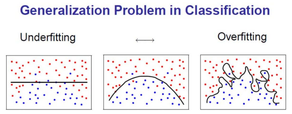
With any classifier there is a risk of underfitting or overfitting the training data which this training method would not be able to test for. Overfitting is where the algorithm is so finely tuned to the dataset that it is unable to make the generalisations on the data required to classifier unseen data accurately.

Overfitting

Therefore, the most basic testing method is to split the training set into halves. The first half is used to train the classifier, the second half is used to test the classifier (as we know what the correct answer is). The advantage of this is that we can quickly get a percentage accuracy for our classifier. The disadvantage is that we’re testing a half-trained classifier so it doesn’t give us a good indicator of how it will perform with the full training dataset.

This brings us onto cross-validation. This is where the training dataset is split into n-subsets, testing performed on each one and the results averaged in order to get a better estimate of classification accuracy. It helps to counter-act overfitting and underfitting.

For this problem I chose 2-fold cross-validation as the testing approach to implement. For this, I continued to split the training dataset into two halves. The classifier was then trained on the first have and the second half was used to test accuracy. Then, the classifier was reset and trained on the second half and tested on the first half. These results could then be averaged to get a better accuracy figure.

Optimisation

There are two main tasks that our classifier has to undertake, and for those familiar with big O notation, these are their complexities:

Learning/Training (Offline)
- Importing our training data into the system so that it can “learn” and be ready to classifying unseen data.
- This process has big O notation of O(n) where n is the largest of either the size of the dataset or the number of different words x number of categories. In most cases n will be the size of the training dataset.
Classify (Online)
- Processing a document against the trained system and producing a result.
- O(n) where n is the length of the document x number of categories.

While we have processing power, memory and storage in a greater abundance than ever, all have the potential to become limiting factors when it comes to machine learning. In practice, I tackled these challenges with a range of optimisation techniques with the aim of reducing the value of n without significantly reducing the accuracy.

Reducing Resource Usage

The larger the training dataset, the more accurate our algorithm is likely to be. Unfortunately, the larger it is, the more RAM and longer it takes to train and question our classifier (albeit on a linear scale as discussed above). So I considered options for minimising the size of the dataset while maximising its accuracy. On a rudimentary level, the process discussed above of prioritising the documents to train was one way that I achieved this. Aiming to get breadth in the training dataset before getting too much repetition in a single category that didn’t add benefit.

Another technique that can be used is that of Stop Words. These are words or terms that we are declaring in advance that our classifier should ignore. A black list that removes them from the equation.

For my situation, I experimented with selection the most popular 0.1% of words and marked them as stop words to remove them from the equation. The results were:

Peak memory usage before stopwords
- During learning and testing: 211MB
- During classifying entire dataset: 475MB
Peak memory usage after stopword
- During learning and testing: 172MB
- During classifying entire dataset: 422MB

The Bag of Words technique provides a similar solution but from the opposite direction by specifying a set of words or terms that are allowed, i.e. a whitelist. This requires a significant understanding of the underlying data which is not always practical.

Normalisation

Normalisation is a process by which similar words or synonyms are transformed into a single version during both training and classification in order to be able to make connections that would not otherwise have been made. For example consider a clothing sites that each used the word “dress”, “dresses”, “Dress”, “dréss” (for whatever reason). The most basic normalisation process would be to lower case all words entered into the system so that additional correlations and connections can be made.

Stemming is another version of normalisation, where we remove pluralisation and verb endings so that all instances are recognised as the same word, e.g. “dress”, “dressed” and “dressing”.

The Porter Stemmer algorithm is a popular one. Unfortunately, this wasn’t useful for my task. Firstly, because it’s not readily available for many languages but secondarily it would require us to know which language we are dealing with in order to choose the right stemmer. This is clearly not an option when trying to classify the language in the first place!

This has no little effect on the resource consumption (other than CPU) of the classifier but is done with the aim to improve on accuracy that otherwise would have required further sample data to identify the similarity.

Tokenisation

For this classification we’re using 1-grams, i.e. each token is made up by a single word, you could increase this, e.g. 2 words per taken (2-gram). Then the additional context serves as more of an identifier. My understanding is that this typically would mean that you would need a larger sample when compared to 1-grams but is typically preferred.

Alternative Algorithms

I primarily focussed on Naive Bayes as a well documented, popular and well regarded algorithm but there are many more out there that take different approaches which can suit different problems. I experimented also with Support Vector Machine (SVM).

The library by Cam Spiers made this as easy as instantiating a different classifier and the rest of my approach still worked.

The results were quite astounding. With the same dataset and testing technique, SVM performed very poorly when compared to Naive Bayes.

I’m not sure if this is partly to do what problems SVM is more suited to solving or whether perhaps it’s slow starter and that with an larger training dataset it’s accuracy would increase in this test space. It’s something that could be tested for.

Conclusions

For my classification problem, almost 3000 sites were trained and he classifier achieved 93% accuracy on identifying languages. For content type classification it is accurate only 44% of the time.

In terms of reviewing and researching Naive Bayes, it has been found that:

It has reasonable (linear) performance when considering big O notation
In terms of accuracy, Naive Bayes is considered generally good at classification decisions but is over-confident in its decisions.
It is capable of withstanding noise introduced during training as false classifications are cancelled out.
It struggles when tackling problems that have a large number of possible solutions. It works best with just a few possible results.
When comparing the language classification to content type classification, the above problem is worsened by the fact that the number of shared words between content types when compared to languages is much greater - causing more confusion.
Anecdotally, I also found it far more difficult to classify content types during the training period. I hypothesis that better results would be achieved by reducing the number of closely related categories, e.g. Home and Garden and Furniture.
You can always do more training. The “best” machine learning technique will have the greatest accuracy for the same sample.

Next up is to experiment with alternative machine learning algorithms, probably via the AWS service. Particularly ones that provide the ability for multiple features and weighting between them. For instance, in my classification problem, passing in the TLD with a weighting factor would help to improve language prediction accuracy.

Post-script

For those interested in receiving news updates on exponential change, including those achieved through AI, I recommend Azeem Azhar’s newsletter.

Thanks also to Cam Spiers, without his library, my understanding of and experimentation with machine learning would have been even further belated.